Historical Cattle Price Cycle Effects on the Heifer Purchase Choice
December 2014
The beef cattle price cycle is one of the most recognized cycles among agricultural markets (Rosen et al 1994). Many have studied its effects and some claim it may be used to the producer’s advantage, such as Harlan Hughes, a retired North Dakota Livestock economist and current contributing editor to Beef magazine. This short essay leaves the discussion about the cycles, existence, relevance, and usefulness for another time, but will discuss the effects that a future cycle might have on the value of purchasing replacement females/heifers.
Let’s assume two different average purchase prices for pregnant ready-to-calve beef replacement heifers. A low price of $2,000.00 and a higher one of $2,500.00. The prices for such animals would likely have a range, which we designate as a truncated normal distribution with more than a 98% probability of lying between $1,800.00 and $2,200.00 and between $2,300.00 and $2,700.00 respectively for the two price ranges. Furthermore, the expected cull rate for these sample cows will be fixed at approximately 20%, where the age distribution of the herd is enumerated in Table 1 (below).
| Cow Age | Cow Numbers | % of Herd |
|---|---|---|
| 2 | 60 | 20.0% |
| 3 | 51 | 17.0% |
| 4 | 46 | 15.3% |
| 5 | 36 | 12.0% |
| 6 | 29 | 9.7% |
| 7 | 21 | 7.0% |
| 8 | 17 | 5.7% |
| 9 | 14 | 4.7% |
| 10 | 12 | 4.0% |
| 11 | 9 | 3.0% |
| 12 | 5 | 1.7% |
Age distribution is important and can have a huge effect on the resulting net returns and will be explored in a later work. The reason age distribution is important is that it is used as a proxy for heifer life and production expectancy. Assuming the cows are profitable, the longer a cow is present in the herd the greater her contribution towards her initial cost and longevity increases her value since she is more productive.
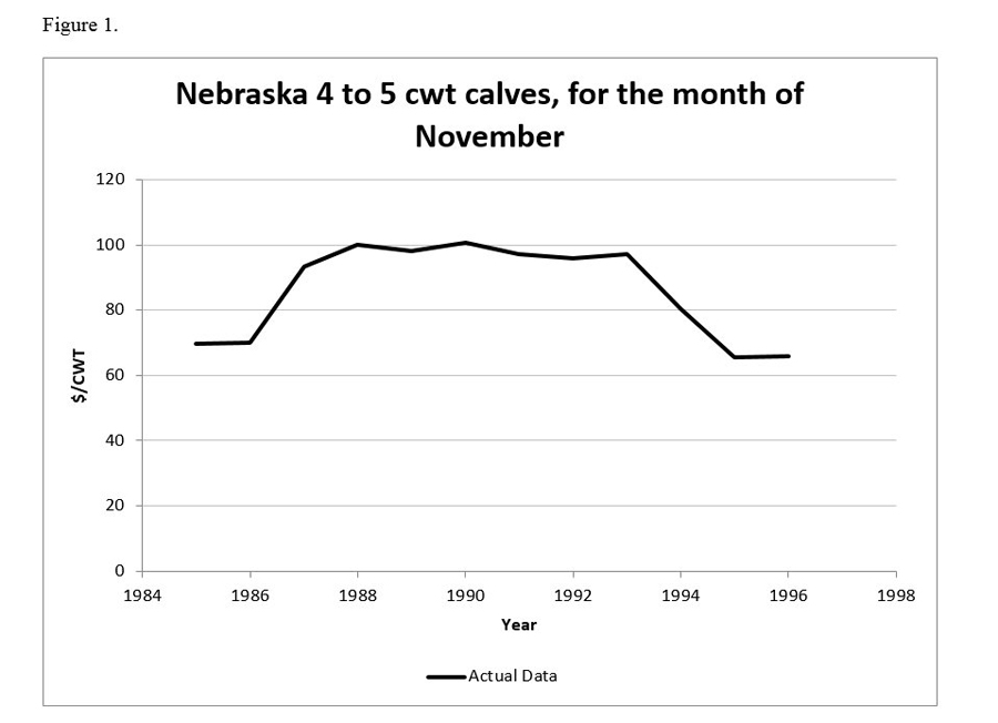
The first step in simulating the price cycle effects is to decide on a methodology that accurately portrays the relevant characteristics of that cycle. In this case, two price cycles were created that mimicked the historical period of 1978 through 1996 using annual percent changes in average monthly prices for the month of November. From previous work (Stockton et. al. 2007) the length of the price cycle has been estimated to be close to 10 years or 124 months. This is convenient since it is also the approximate length of a cow’s productive life, in our simulation 11 years. These cycles were initiated in 1985 and 1978 from average monthly historical prices for 400 to 500 lb. calves in Nebraska. Figure 1 (below) graphically represents the actual prices for that period.
Once the simulated price cycles are defined, they were used in two scenarios where beef cow replacement females are purchased. Scenario 1 replacement values range at the low level, $1,800 to $2,200 per head with an average costs of $2,000. Scenario 2 replacement values range between $2,300 and $2,700 per head and have an average cost of $2,500. In both scenarios purchased animals are identical except in price. Both the weaned calves and any sale of culled cows are valued based on November prices. Production cost, without purchase, opportunity, or depreciation were set at $800 per cow for the first year and increased by 1% annually over the next ten years. Cull cows sell for 44% of the value of the current 400 to 500 lb. calf value, each on a cwt basis. Calving rate averages 90% with a low of 88% and a high of 92%, with weaning weights averaging close to 500 lbs. All of this information was entered into the “Cow Purchase Cow-Q-Later” spreadsheet (available from the author with all of the relevant data) which provided simulated averages of 500 randomly drawn outcomes. The resulting net returns which consider the time value of money, depreciation and investment costs are summarized in Tables 2 and 3 (below).
| Early Entry | Mid/Late Entry | |
|---|---|---|
| Average Breakeven Value | $2,281.03 | $1,566.55 |
| Average Age to Positive Return | 5 | 11 |
| Average Age of the Cows in the Herd | 5.06 | 5.06 |
| Average Net Return/Cow | $408.20 | -$380.81 |
| Early Entry | Mid/Late Entry | |
|---|---|---|
| Average Breakeven Value | $2,305.40 | $1,568.91 |
| Average Age to Positive Return | 6 | 13 |
| Average Age of the Cows in the Herd | 5.07 | 5.05 |
| Average Net Return/Cow | -$134.44 | -$967.80 |
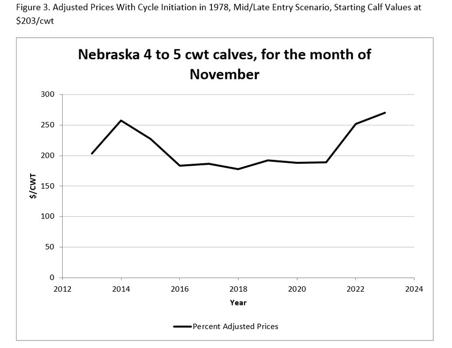
The electronic simulation is done by first substituting more currently relevant prices for the historical ones. The percent changes from a beginning or initiation point are used to calculate the new cwt prices and are illustrated in Figures 2 and 3 (below). The Figure 2 graph has a similar shape as Figure 1 (above) due to the fact the start point or date 2013 corresponds to 1985. This cycle represents purchases made as an early entry into the upward trending part of the cycle. Figure 3 or the adjusted 1978 cycle represents purchases made mid/late cycle entry when it is peaking and then receding, and is initiated seven years earlier. Each cycle represents the changes in heifer/cow value at different time periods along the same future price period.
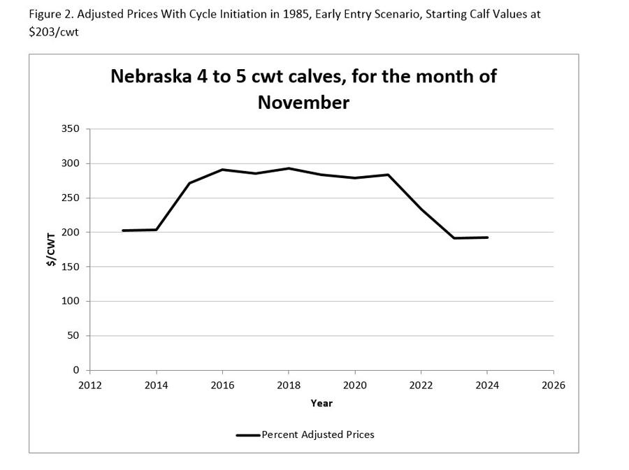
Both the early entry and the mid/late entry cycles are initiated with a $203/cwt price for the first November 4 to 5 cwt calf prices. This price is intended to be reflective of the pricing level of 2013. Forecasts for each of the cycles subsequent ten years follow the pattern set as a percent change in price depending on the previous year’s price. That is the November 1985 and 1978 price are multiplied by their respective percent changes observed historically and become the adjusted 2014 price for their respective cycles. This process is repeated sequentially for all of the years over the life of the cow.
Results
Tables 2 and 3 when averaged indicate a $725.49 average difference in breakeven values between the two cycle shapes. Given the magnitude of the annual price changes heifer purchasers could pay more than $700 more for replacement heifer if they knew that they were experiencing the early scenario verses mid/late scenario. Note that breakeven value is defined as that value that producers could afford to pay for a replacement female with the expectation of zero economic profit. Where zero economic profit, is that level of net returns that would just keep producers satisfied and in business over time, but no more.
In this case the early cycle prices are forecast to reach a pinnacle in 2018 (1990 on the graph), whereas the mid/late cycle reaches a low in the same forecast year. Average net returns given the $2,000.00 average price paid for replacements in the early entry cycle scenario result in an average positive $447.74 and a negative $414.88 for the mid/late entry scenario Table 2. These values are even lower for heifers purchased at the higher $2,500 average price and reach an average high of -$134.44 for the early entry scenario and a low of -$967.80 for the mid/late entry scenario. Making the $2,500 average purchase price have a negative net return on average (the price was higher on average then the return).
Conclusion and discussion
This result highlights several points worth discussing.
First the profitable heifer purchase decisions require some consideration of more than current prices. Having some idea of future productivity, including longevity is essential to a respectable estimate of heifer value. Longevity plays a huge role into the favorability of the investment as illustrated in the case of the early entry scenario the $2,500 purchase price resulted in requiring an additional year of productivity to reach a breakeven point over the $2,000 purchase price, 6 verses 5 years. This is noteworthy since the average cow in the sample herd is about 5 years old making it more likely that purchased animals will not reach the breakeven point at the higher purchase price. In the case of the mid/late entry scenario two additional years of production are required to breakeven for the higher priced heifers verses the lower priced. But in this case either priced animal does not breakeven until after they are 11 years of age, which in this herd means an average of about 3% of the cows in the herd; which is an indication they (the cows) are 97% likely not to reach the breakeven point.
Given the uncertainty associated with this decision as demonstrated by this example it is important to consider the price that is paid for the replacement or additional animals, to consider the effect of future price expectations, and the longevity of productivity needed to make the investment have a positive outcome. Buying short-lived high-priced cows is analogous to investing in ice on a hot day without refrigeration; cool for a while, but soon to be gone.
While nothing can be said about the surety of the price cycle, the fact that it has persisted is a likely indication that rising prices are likely at some point to recede, making the timing of the decision of when to purchase, how much to pay when you do purchase and how many to buy requires some careful thought. Purchases made early in a cycle like the one used here are more likely to achieve a positive net return while those made later in a cycle provide less opportunity, but even when purchased at the correct time in the cycle animals must be bought at an affordable level.
Rosen S., K. M. Murphy, and J. A. Scheinkman, Journal of Political Economy, June 1994, Vol. 102, No. 3, pp. 468-492. https://ideas.repec.org/a/ucp/jpolec/v102y1994i3p468-92.html (IDEAS bibliographic database dedicated to Economics)
Matt Stockton
Nebraska Extension Ag Economist