Buying a beef herd bull is a long-term investment. The right bull at the right price can provide gains in herd productivity and increased business stability. The current historically high cattle prices may or may not continue into the foreseeable future, but if history is any indication, the lows will soon follow the highs. When and/or if this happens, producers face the risk of having overpaid for their breeding animals.
Whether you’re managing a smaller operation or a larger herd, the price you pay for breeding bulls can significantly impact productivity, efficiency and profitability. To ensure production and business success, it is essential to understand the financial implications of merit-based bull purchasing while balancing cost limitations with operational goals.
This short discussion lays out the basic drivers behind valuing individual bulls, using an excel spreadsheet to do the math, and provides a ranking based on the users’ criteria. It is intended to be straight forward, easy to use, and reflect outcomes based on individual preferences.
Part 1 (Input Information)
The spreadsheet is designed to define, develop and create the information needed to rank bull value on a per calf basis. The following topics list the information necessary to do this.
In the Beef Bull Value “Cow-Q-Lator” (BV-CQL), there are a series of 13 questions. These questions are designed to capture the relevant information needed to make an objective evaluation of bull value.
The topic areas are:
- An estimate of annual cost of owning and keeping the bull (feed, care, veterinary, management, facilities, etc.)
- The current purchase value, cull price of the bull(s) you own
- The bull’s expected productive life as a herd sire
- The number of cows expected to be bred by individual bull(s) annually
- The percentage of cows bred expected to wean a calf (weaning rate)
- The purchase value and cull value of the bull(s) to be purchased
- Interest rate of borrowed money
- The bull’s chance of dying during a single year
- The bull’s chance of being injured during his time in the herd
- The contribution measured in dollars that each new bull will add to each calf compared to your current bull(s)
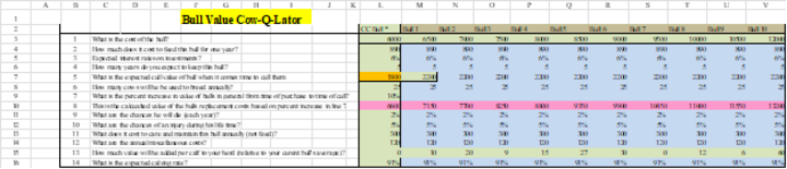
These factors are listed in the BV-CQL 1.0 file on the “Program” worksheet tab (lines 1 through 16, columns A through J, as illustrated in the picture labeled Figure 1).
The worksheet has room to capture and evaluate eleven bulls including the CC Bull* (current, baseline or benchmark) and ten purposed purchase animals. The value for the above information need not be difficult to obtain, even if this means they are estimates generated from prior experience and through experiments. It is important to remember that the more precise the information, the more accurate the comparison.
In Figure 1, the green cells are for data entry (lines 3 through 16, column L, and columns M through V for rows 3, 15 and cell M7). The individual columns, M through V, capture individual proposed bull purchase information. Column L is used to enter the information requested by the adjacent questions and is copied to various cells required in the calculations. The L column is designated as the current bull, CC Bull*, and is the benchmark for all bulls being considered for purchase. For convenience, the columns that are highlighted in blue are repetitive and copy the information entered in the L column. The pinkish colored row is a calculated value based on entered information and fills automatically unless it is overwritten. The orange cell is the current cull value with the adjacent green cell (M7), indicating the expected cull value of the bull(s) being considered for purchase. The blue cells imply that all bull costs, longevity, numbers of cows bred, etc. are identical. Only two rows have individual column differences: row 3, purchase price and row 15, the bull’s expected contribution to calf value. The blue cells may be changed individually but to do so will overwrite/destroy the copy function of those cells. To preserve the integrity of the original spreadsheet, it is recommended that the user make and use a saved copy of the original excel spreadsheet using a different name prior to making those changes.
Part 2 (Output Information)
There are a total of eleven output categories. Columns A through J provide the appropriate descriptions, while L through V have the calculated values listed by individual bull.
The outcomes include:
- Annual depreciation with no death or injury costs
- Annual death loss value
- Annual injury loss value
- Annual interest cost/value on investment
- Annual total maintenance costs (with interest)
- Annual interest cost on feed and other cost
- Annual total or cumulative cost
- Cost per cow covered by the bull
- Bull cost for each calf weaned
- Expected cost per weaned calf and added value by the bull
- The change in cost of the proposed purchased bull versus the benchmark bull
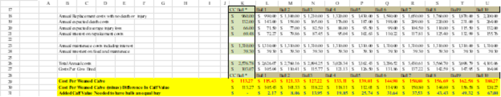
These outcomes are listed in the picture shown in Figure 2. Each outcome in the BBV-CQL listed in the program’s worksheet are listed in the same order described above. However, they may vary in their wording. The first seven cost items in the above list (A through G) focus on common animal costs. The next three items (H, I, and J) show individualized cow or calf cost, and the outcome (K) measures the various cost differences of each bull considered for purchase versus the CC Bull*. This portion lists the outcome of the information entered in the top portion of the worksheet and requires no entries. The green color in column K is used to designate it as the column containing the current bull cost.
Part 3 (Focus Factors)
While each of the thirteen factors listed in Part 1 contribute to calf breeding costs and all are important, there are six which stand out as being significant to individual bull cost differences. The six factors are expressed in questions 1, 4, 5, 6, 13 and 14 (see Part 1).
- Purchase value – has direct effect on cost. As bull purchase price increases, under the same usage and productivity levels, each pregnancy and weaned calf will cost more to produce. Question 1.
- Productive lifespan length – there is an inverse relationship between purchase costs and depreciation length. A decrease in productive lifespan will increase the $/calf cost as annual depreciation costs increase. Question 4.
- Cull value – as cull value increases, depreciation expense declines, reducing the net annual costs and $/calf costs. Question 5.
- Number of cows bred – with no increase in bull cost, increasing the number of cows bred spreads the fixed cost across more animals, resulting in a reduction of $/calf- assuming calving rate, productivity remains unchanged. Question 6.
- $/calf contribution – the more value that can be derived from calves of a specific bull the more the value of that bull is increased, since the added purchase cost is compensated for, making the difference between costs and revenue shrink. Question 13.
- Calving rate – calves are the primary source of revenue. If the same number of cows have more calves on the ground from the herd (improved calving rate) due to the bull. The greater will be the return from the bull. Question 14.
Part 4 (Examples)
High vs. Low priced bulls
When considering two bulls for purchase:
- One is priced high at $10,500/hd., (Bull 9 in Figures 1 and 2) and the other is priced at $7,000/hd. (Bull 2 in the same figures).
- In this instance, each bull is expected to cover 25 brood cows annually, have an expected 5-year productive life, an annual chance of death of 2%, a 5% chance of being injured during their productive life, with cows having a 91% calving rate, and an annual maintenance cost of $1,310/hd., as captured in Figures 1 and 2.
- Bull 9 has a $37.55/hd. higher cost to breed each cow and a $41.25/hd. higher cost per weaned calf compared to Bull 2.
- Bull 2 has a lower upfront cost. Does this mean he is the better buy? To determine this requires further information about the resulting value of the calves produced by each bull and their contribution to the operation.
- For the purposes of this example, it is assumed that the buyer’s objective is to have the highest possible annual net return or profit. Knowing that calves born to Bull 9 are $41.25/hd. more expensive makes the calculation easy. If this bull’s calves on average weighed an additional 20 lbs./hd. than those of Bull 2 with an average calf value of $3.00/lb., Bull 9 on average adds $60/hd. more revenue than Bull 2. Given that maintenance cost is no different between the two animals, Bull 9’s net return is $18.74/calf more than Bull 2. This makes Bull 9 the more profitable choice.
- In this example, heavier weaning weights are a direct and easily observed difference. However, where calf value is deferred to some future date (e.g. genetic potential, cow longevity, etc.), it is not easily recognized. In these cases, the unmeasurable and undefinable should be considered in the decision process with recognition that the added cost of the bull has a probability of achieving the hoped for future value. This risk has a cost and should be recognized accordingly.
- There are times when bull cost cannot be justified upon direct returns and require the acceptance that those costs have a high risk. The question may become, “Can I afford the risk”? This is sometimes the case when bulls are purchased for their so-called genetic merit when it is difficult or impossible to quantify the value of an individual bull’s impact on future productivity and value. Investing in the future is important but shouldn’t come at the cost of insolvency and high levels of risk. Each bull’s expected contribution, if possible, should be objectively recognized and considered in light of the operation’s capacity to absorb the added cost without putting the operation into financial jeopardy.
Increasing Cows Per Bull
If the number of cows per bull is increased from 25 cows/bull to a higher level of 45 cows/bull, the cost per calf declines proportionately. Using the above information and increasing the cow/bull ratio to 45 in the BBV-CQL results in the cost per weaned calf being reduced drastically as is shown in Table 1 below. With 45 cows per bull, cost per weaned calf is $64.13 for the $6,500 bull and $100.15/calf for the $12,000 bull. For the same bulls servicing 25 cows, the cost per weaned calf increases to $115.43/calf for the $6,500 bull and $180.27/calf for the $12,000 bull.
Table 1. Comparison of 25 cow/bull ratio to a 45 cow/bull ratio, data from previous example.
CC Bull cost of covering 25 cows is $113.27 (Figures 1 and 2)
| Bull Cost | $/calf weaned (45/1) | $/calf weaned (25/1) |
| $6,500 | $64.13 | $115.43 |
| $7,000 | $67.40 | $121.33 |
| $7,500 | $70.68 | $127.22 |
| $8,000 | $73.95 | $133.11 |
| $8,500 | $77.23 | $139.01 |
| $9,000 | $80.50 | $144.90 |
| $9,500 | $83.78 | $150.80 |
| $10,000 | $87.05 | $156.69 |
| $10,500 | $90.32 | $162.58 |
| $11,000 | $93.60 | $168.48 |
| $12,000 | $100.15 | $180.27 |
Practical use of the tool using sale catalog information
One application of the Cow-Q-Lator is to value bulls in a sale catalog.
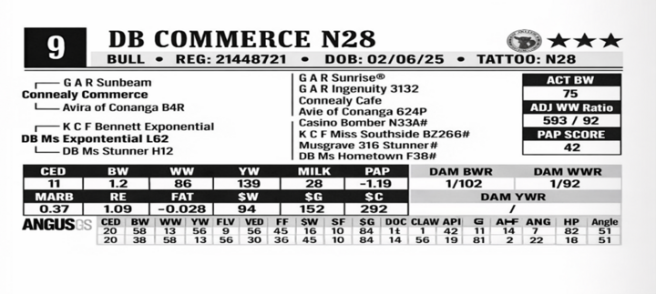
Looking at the sale catalog data in Figure 3, we see $W of 94 for DB Commerce N28. There is also other information that we could use, but we will focus on $W for this example.
From the picture, the sale catalog shows this bull with a $W score value of $94. Our present herd sire, CC Bull*, has a $W score value of $75. The difference is $19. This value is put into the BBV-CQL, and the output captured is presented in Table 4.
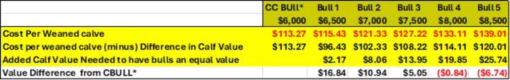
By varying the bull’s value, his breakeven with the current bull cost can be estimated. The values used in this example range from $6,500 to $8,500. As bull price increases, cost per weaned calf rises from $113.27 to $139.01. Without considering the $19/hd. $W, all these bull values exceed the current cost. But after subtracting the $19/hd., Bull 4 comes closest at an adjusted calf cost of $114.11, costing $0.84/hd. more. The adjusted cost per weaned calf ranges from $96.43 to $120.01. The Bull 1 price is $2.17/calf more than my current cost but $19 worth of $W is gained. This analysis assumes that the purchased bull and the CC Bull* are equal in all other ways in terms of their calves, and they only differ in the $W characteristics. So, for this example the breakeven is somewhere between $7500 and $8000 priced bull.
Conclusion and Summary
There is no one-size-fits-all answer to what constitutes a "good price" for a bull. The right price depends on multiple factors, such as genetic value, herd objectives, calf marketing potential, cow longevity, etc. Purchasing a beef bull is a long-term investment that affects herd productivity, cost structure, and financial risk for multiple years. The UNL Beef Bull Value Cow-Q-Lator (BBV-CQL Version 1.0) provides producers with a practical, objective framework to evaluate bull purchases based on their true cost per weaned calf rather than purchase price alone.
This tool demonstrates that as bull prices increase the cost per calf also increases. To pay the higher price, you need to get added value from the bull, if not it is costing you more money to produce each calf. Factors including bull purchase price, productive lifespan, cull value, calving rate, number of cows bred, and added calf value are the primary drivers of economic differences among bulls. Even small changes in these variables can significantly alter outcomes.
Examples are given to show that a higher-priced bull can be the better investment when additional calf value exceeds the added cost of ownership. Conversely, when expected value is uncertain or delayed, higher bull prices increase financial risk. This risk must be carefully weighed against an operation’s ability to absorb or mitigate that risk. Increasing cows per bull, when biologically and managerially appropriate, is one of the most effective ways to reduce cost per calf and justify higher-valued bulls. Bull catalog information can be used to pre-access bull value differences and affordability.
Ultimately, there is no single “right” bull price. Each operation is unique with varying circumstances and objectives. The right price depends on herd goals, marketing strategy, genetic priorities, and risk tolerance. By using the principles embedded in the BBV-CQL, producers can align bull purchasing decisions with their operational objectives, improve cost control, and make more informed, defensible investments that support long-term profitability, sustainability and goal attainment.
Resources
Download the Bull Value Cow-Q-Lator here. https://cap.unl.edu/livestock/tools/
View the webinar to learn how to use the Bull Value Cow-Q-Lator. https://cap.unl.edu/bull-value-webinar-2026/