This is a summary of the sixth annual beef cow replacement value forecast for Nebraska. The entire forecast can be found at this link, and past summaries are also available on the Farm¢ents site. The information presented in the forecast is intended as a guide to modify, depending on each producer’s circumstances, expectations of future production costs, and cow and calf values. The forecasted price and cost variations come from the University of Missouri Food and Agriculture Policy Research Institute (FAPRI) 10-year projections and the UNL 600 cow herd budget for Central Nebraska. Biological measures, such as cow size, weaning weights, etc., are relationships derived from the Gudmundsen Sandhills Laboratory cowherd.

Replacing females in the cow herd looks differently for each farm and ranch. Value for both retained and purchased replacements generally depends on the following factors:

• Longevity - the length of time the replacement animal remains in the herd
• Productivity - annual expectations of calf size, calf value and costs over the replacement’s productive life
• Genotype and phenotype - the animals physical compatibility with the production system and performance goals of the ranch
• Operator goals and management style
• Financial standing, specifically debt related to cow purchases
• Environmental conditions of the operation (drought, fire, etc.)

Leaving the other considerations to those making the replacement decisions, this forecast focuses on two main factors:

1. Annual cost of production per cow. Authors used the University of Nebraska at Lincoln (UNL) Cow Cost Cow-Q-Lator to help calculate three levels of costs: low (Lo), Mid, and High (Hi). Livestock budget information from Kansas State and UNL contributed to these calculations. Costs relate directly to the 2022 Nebraska state average low, median, and high pasture rental rates for the sandhills area found in UNL Agricultural Economics department’s 2021 Nebraska Ag Real Estate Report. Three levels of annual production costs per cow were identified as $747.41/cow (Lo), $881.71/cow (Mid), and $992.54/cow (Hi).
2. Average historical replacement rates. This is the number of heifers needed each year to replace culled cows or cull rate, while keeping the same cow herd number. This number can be used as a proxy measure of average cow longevity. This forecast evaluated 14, 20, and 28% replacement rates.

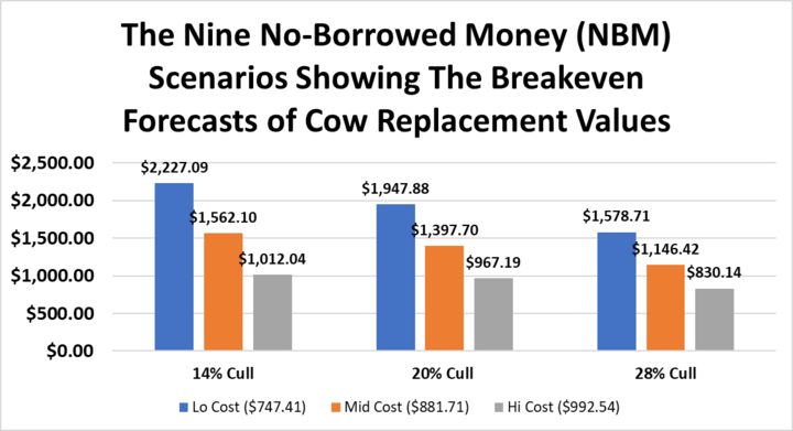
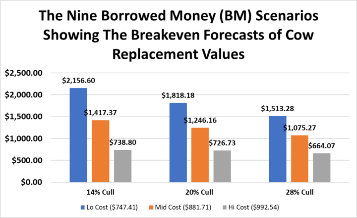
The forecast looks at the three levels of cow costs at each of the three replacement rates. The values shown in Figures 1 and 2 are the amounts at which producers could purchase replacements and still break even at each combination of cow costs and replacement rates. The difference between the figures is the purchase price if paying in cash (Figure 1) versus borrowing the money (Figure 2). The simulations require the cows to have a purchase value. CattleFax data was used to get an annual average of $1,705/hd. The model was allowed to randomly draw a cost of $1,866/hd and $1,524/hd, using a normal distribution. (See Addendum 1.) Borrowing money to help pay for replacements also reduces the amount that can be paid for replacements, captured in Table 1. The simulation breakeven forecast results are reported in Figures 1 and 2. As expected, costs of production and replacement rates affect replacement heifer value.

This year’s forecasts are not much different than last year’s report for the nine NBM forecast. Three of these scenarios (Lo) were higher than last year’s breakeven value, while six Mid and Hi were lower. Borrowing money to purchase heifers also reduced average break even. Production costs were higher than last year. Projected future costs are also elevated, but so are future animal values, compensating for the higher costs in the Lo cost scenario. However, in the Mid and Hi cost scenarios, the higher price of calves did not increase what could be paid, instead the higher cost decreased the breakeven value. Increasing productivity without altering costs would result in greater revenue, which would not be accounted for in any of the scenarios. Therefore, the accuracy of the forecast is dependent on how closely an operation’s productivity and revenue match those specified in the model. Productivity changes, including calving rates and calf growth rates, among others, would change the results. The simulation was built using a March calving herd with an average calving rate of 92%. Revenue changes also play a role in altering what one can pay for a replacement. Demand and supply shifts that alter cattle price also have an impact on replacement heifer breakeven value. Higher calf prices lead to higher breakeven values, while lower prices lead to lower breakeven values.

A positive outcome in purchasing replacements over time comes down to the purchase or raised animal’s ability to return as much or more value than was paid, and this is only accomplished if the operation selects the right type of animals, at the right price, and the right time. Purchasing a replacement heifer involves risk because her longevity, productivity, and cost are unknown.

When raising or purchasing replacement heifers, each heifer’s value is based on her ability to stay in the herd and the producer’s ability to manage that productivity, control costs, and use the market to their advantage. Applying these principles is key to making an operation more profitable and resilient.

For more information, please plan to attend the UNL Center for Ag. Profitability webinar on Thursday, January 12, at noon, which will be hosted by the authors of this article. 

Interviews with the authors of BeefWatch newsletter articles become available throughout the month of publication and are accessible at https://go.unl.edu/podcast.