What is a respectable value of a beef replacement heifer for the coming 2019-2020 production season? This can be a complicated choice, but a vital one that requires some clear thinking. It is important to have a handle on this value since future prosperity partially depends on it. Pay too much and future profits and net worth will suffer. Non-participation in the market is not likely to be an option since cow numbers are necessary to maintain productivity. To provide a starting point, the University of Nebraska Beef Economics team makes annual forecasts of heifer values using publically available projected price and costs scenarios (UM FAPRI annual 10 year projections).

While the selection of replacement animals in a herd of beef cattle may differ from ranch to ranch, there are three factors seen by the authors as critically important that affect their value as replacements. These factors apply for both retained and purchased brood heifer replacements.

These general factors are:

• Longevity - the replacement heifer’s ability to stay in the herd as a productive unit
• Costs verses Value – both current and future expected difference between costs and revenues (calf price and costs differences over the heifer’s productive life)
• Genetic and phenotypical compatibility with herd mates and operators goals and management style

Since it is difficult to anticipate and quantify all the possible conditions, types and choices that might occur, three general cost scenarios and three herd cost types were used to create a total of nine different breakeven value forecasts. The resulting nine forecasts are the product of 1000 possible outcomes from probable price and production variations.  Outcomes will vary by producer depending on unique circumstances, level of productivity, genetic differences, management styles and available resources.  

Three levels of heifer costs were identified on a per heifer basis for the initial 2019/2020 calving season and then adjusted in percent terms to match those forecast by the Food and Agricultural Policy Research Institute (FAPRI) at the University of Missouri. Three Nebraska annual brood cow production costs in the Nebraska Sandhills (Nebraska Statistical District, North) were estimated. Pasture rental rates were those reported by the UNL Agricultural Economic Department’s 2019 Nebraska Ag Real Estate Report. The low cost producer was estimated to have an average annual cow cost of $629.50/hd.  without replacement, depreciation or death loss.  The middle 2020 heifers were expected to have a cost of $712.10/hd. This value is very close to the FAPRI costs estimate of $717.32/hd. The 2020 high cost herd was estimated to be $822.70/hd. These forecasts relate directly to the reported pasture rental rates of the region, a low of $47.45 per cow/calf pair, high of $70.95 per cow/calf pair and an average rental fee of $57.90 per cow/calf pair. These are summer pasture rates.

FAPRI forecasts both production costs and prices for cattle for each of the ten years listed in their report. As indicated, these costs were used to create an index to adjust the three initial cost levels to the appropriate year in the forecasting model.

Revenues are based on FAPRI calf and heifer forecasts for March born calves sold in the late fall for the next 10 seasons. The animal productivity information was derived from ranch records of the University of Nebraska Lincoln’s Gudmundsen Sandhills Laboratory (GSL).

Capturing the longevity of any one animal is a difficult proposition at best. Therefore, the idea that the current herd production performance is the best predictor of future performance was adopted. Since, longevity is one of the keys in valuing any particular animal, a statistical model of life expectancy and productivity was created using the GSL data for three different expected cull rates: the lowest is a 14% cull rate with an average cow herd age of 5.88 years (older cow herd), the mid cull rate is 20% with herd age averaging 4.85 years (medium aged cow herd), the third cull rate is 28% with a herd average age of 4.00 years (young cow herd).

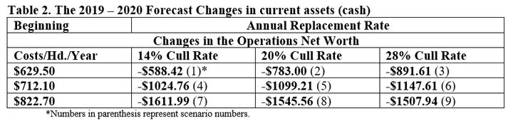
Results are reported in two ways: 1) As the simulated average breakeven value, forecast by scenario and 2) Changes in (current assets) where replacements on average cost $1650/hd. It was assumed for simplicity that replacements were purchased with cash.

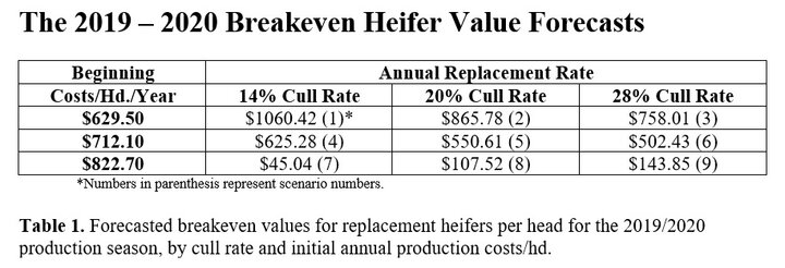
The low rate of replacement (14%) and the lowest cost of annual production ($629.50/hd./yr.) has the highest available replacement value of $1060.42/hd. The highest replacement rate (28%) with the highest production cost of $822.70/hd./yr. had a heifer replacement value of $143.85/hd. Higher cull rates and higher annual heifer costs generally result in lower breakeven values. Heifer longevity, as expected, increases replacement breakeven values. This is also true of costs. However, when costs are at their highest, herds with less culling of older animals, result in those older animals costing more than shorter lived animals. This outcome could be falsely interpreted as indicating higher turnover rates among cows is advantageous. When in fact it indicates simply that losses are minimized by selling cows early when they are going to continue to lose money. This is illustrated in the average breakeven values from scenarios 7, 8 and 9 simulations. Scenario 7 with the lowest cull rate has a lower breakeven value than either scenarios 8 or 9.

The change in current assets forecasted shows how financially damaging overpaying for animals can be and how fast doing so can burn through capital. In this instance, it was assumed that the average replacement heifer was purchased for $1650/hd. Given that the estimated breakeven value for a scenario 1 replacement heifer is $1060.42/hd,   Current assets would on average decrease by about $589 for each purchased replacement ($1650 - $1060.42 = $589). This change in assets ends up on the balance sheet as a decrease in what the owner has in equity. Table 2 below lists the negative effect this overpaying has by scenario.

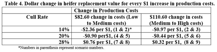
The above information is easily converted into two tables that provide a way to extrapolate an individual producer’s heifer replacement breakeven value. Table 3 shows the effect of cull rate variations by cost level, while Table 4 shows the reciprocal effect of production cost changes by cull rate category.

Using Table 3 and looking between scenario 1 and 2 for each 1% decrease in cull rate, breakeven value on average increases by $32.44/hd. Therefore, breakeven replacement value for a producer having the low costs of $629.50 and a 19% cull rate would be $32.44/hd. higher than $865.78/hd. (20% cull rate breakeven value) or $898.22/hd. breakeven replacement value. The same decrease in cull rate between scenarios 7 and 8 would result in the opposite effect; breakeven value would decrease by $10.41 to $97.11/hd. There are many possible combinations where individual cull rate effects can be extrapolated from the information provided.

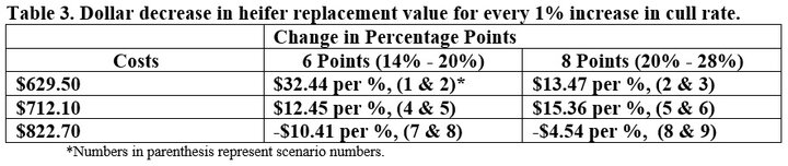
Table 4 can be used in a like manner and is useful in extrapolating the effects that different production costs have on replacement value. For instance, a 14% cull rate with a production cost of $639.50/hd. ($10 more than the low costs) reduces the $1060.42 by $23.60/hd. making the extrapolated breakeven replacement value $1038.82/hd.

Heifer Replacement Breakeven Value Outcomes (Possibility Curves)
The next three figures show each of the nine scenarios grouped by the three costs, low, mid and high. The horizontal axis of each figure shows dollar values representing individual heifer replacement breakeven values. Figure 1 ranges from -$300/hd. to $2300/hd. and depicts scenarios 1, 2, and 3.

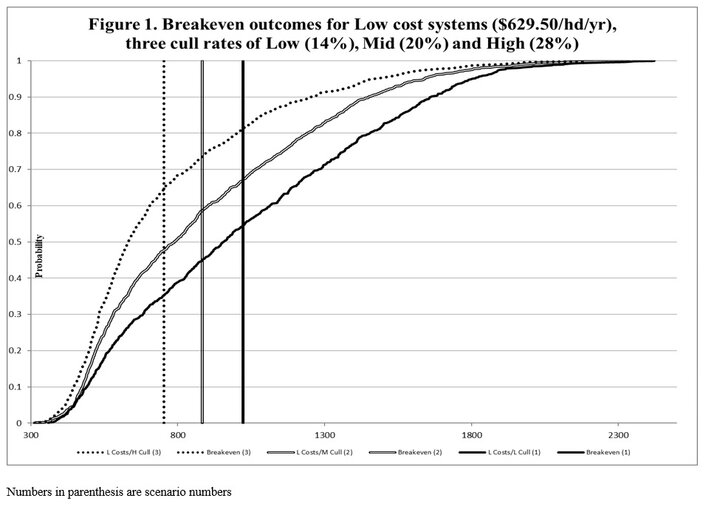
The curved lines are outcome lines and represent the many different breakeven values of the 1000 simulated heifer purchases for scenarios 1, 2, and 3 with their vertical companion lines at the average breakeven value of $1060.42 (1), $865.78 (2) and $758.01 (3), respectively.  Each of the three figures are useful in approximating probabilities of a specific heifer replacement value breaking even given one of the nine cost and cull conditions. The vertical axis represents probability estimates. For instance, the 0.5 mark is the 50% level and 0.9 is the 90% level. In scenario 1, less than one percent (0.001) of the breakeven replacement values were $364/hd. or less (lower left corner of Figure 1). Also in scenario 1, an $800/hd. or less breakeven heifer replacement value was predicted to occur about 67% (0.67) or less of the time. Using Figure 1, a producer with scenario 1 costs and cull rate is considering buying a heifer replacement for $1300. It is easily seen from the figure that the $1300 is right of the vertical line for that scenario, indicating that the $1300/hd. exceeds the average breakeven heifer replacement value. Secondly, moving straight up from where the $1300 crosses the horizontal axis to where it intersects the scenario 3 outcome line, approximately at the 0.7 or 70% probability line, indicating this animal is forecasted to not breakeven 70% of the time.  Conversely implying that 30% of the time the $1300/hd. costs would break even or be exceeded.

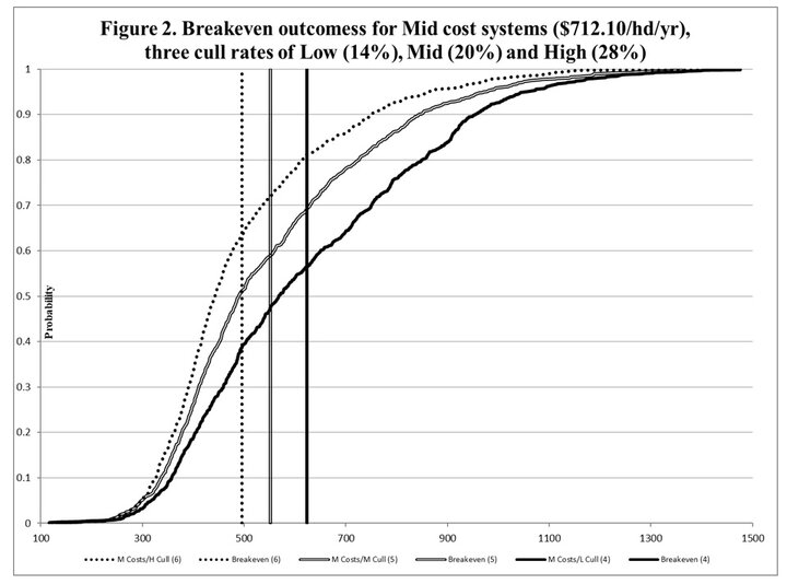
 As production costs increase breakeven values fall; Compare Figure 1 (Low Cost) to Figures 2 (Mid Cost) and 3 (High Cost). To maintain profitability, higher production costs require either an increase in revenue or reduction in replacement costs. Changing cull rates also has an effect on breakeven values as illustrated in each table.  Lower cull rates imply heifers have longer productive lives, thus increasing their value in Figures 1 and 2. In these two figures, decreasing the cull rate moves the outcome curves to the right indicating higher breakeven values. This, however, is not true when heifers are not profitable (costs exceed revenue), as is illustrated in Figure 3, in the high costs scenarios, 7, 8, and 9. For these scenarios, as cull rate increases heifer breakeven value increases. This reflects a loss minimization situation and suggest not buying replacement heifers would be most optimal.

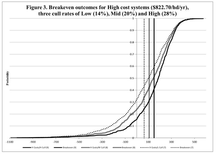
The highest cost scenario shows that the higher cull rate heifers lose less money.  If a producer had a cull rate and cost similar to scenario 9 and paid $300/hd. for replacement heifers, the model forecasts that the probability of breaking even or better is about 20%, or 80% of the time breakeven costs for those replacements would not be realized.

Conclusion
Altering the cost of production or heifer longevity changes the breakeven value of heifer replacements differently depending on the replacement heifers expected life and cost level. From Table 4: A $10 decrease in cost at the 14% cull rate with cost ranging from low to medium heifer replacement breakeven value would increase by $23.60/hd. Whereas the same $10 decrease in the moderate longevity (20% cull rate) herd is predicted to have a smaller gain in heifer replacement breakeven value of $9.00/hd. Likewise, a 2% reduction in a 20% cull rate herd with the lowest cost of production is forecast to increase the breakeven heifer replacement value by $64.88 (Table 3). However, at the high costs ($822.70/hd./yr.), the same 2% decrease in replacement rate is forecast to reduce heifer replacement breakeven value by only $20.82/hd.

So far, nothing has been said about changing productivity which is something like the elephant in the room. Increased productivity without altering costs or changing cull rates will increase the amount that can be paid for replacement animals. Decreases in productivity has the opposite effect. Examples of productivity changes include calving rate, calf size, and calf growth rate. Another factor that changes replacement heifer breakeven value is revenue changes created by cattle prices. Higher prices lead to higher breakeven values, while lower ones lead to lower breakeven values. This last point seems over simplified and obvious, but remember it is complicated by the fact that heifers have a productive life that can span a decade, and that during this productive span prices vary. If prices trend higher overtime, assuming costs are fixed, the purchase breakeven value increases, and vice versa. The economically successful producer is one that on average buys/raises replacement heifers for at least no more than what is needed in net returns.

The relationship between costs and replacement rate is not constant, making production and cost choices critical to consider when paying for replacement heifers. As longevity of heifer replacements increase, average herd age increases and breakeven values also increase except in high cost scenarios. Low cost, low replacement herds are able to afford higher valued replacement costs and take less capital out of the operation. The key to buying higher priced, profitable replacements is based on individual cost structure and herd replacement rate, productivity, and future prices. The key take home message, other than a bottom-line cow replacement value, is that when raising or purchasing replacement heifers, each animal’s value is based on her ability to be productive and durable and the producer’s ability to manage that productivity, control costs and understand and use the market to their advantage. Applying these simple principles is key to making an operation more profitable and resilient. 

Interviews with the authors of BeefWatch newsletter articles become available throughout the month of publication and are accessible at https://go.unl.edu/podcast.